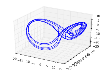
The Lorenz chaotic attractor

This example shows the construction of a classic chaotic dynamical system: the Lorenz "butterfly" attractor. The equations are:

$$ \dot{x}_0 = \sigma(x_1 - x_0) \\\ \dot{x}_1 = x_0 (\rho - x_2) - x_1 \\\ \dot{x}_2 = x_0 x_1 - \beta x_2 $$

Since $x_2$ is centered around approximately $\rho$, and since NEF ensembles are usually optimized to represent values within a certain radius of the origin, we substitute $x_2' = x_2 - \rho$, giving these equations: $$ \dot{x}_0 = \sigma(x_1 - x_0) \\\ \dot{x}_1 = - x_0 x_2' - x_1\\\ \dot{x}_2' = x_0 x_1 - \beta (x_2' + \rho) - \rho $$

For more information, see http://compneuro.uwaterloo.ca/publications/eliasmith2005b.html "Chris Eliasmith. A unified approach to building and controlling spiking attractor networks. Neural computation, 7(6):1276-1314, 2005."

import matplotlib.pyplot as plt
%matplotlib inline

import nengo
%load_ext nengo.ipynb

<IPython.core.display.Javascript at 0x7fdce4678050>

tau = 0.1
sigma = 10
beta = 8.0/3
rho = 28

def feedback(x):
    dx0 = -sigma * x[0] + sigma * x[1]
    dx1 = -x[0] * x[2] - x[1]
    dx2 = x[0] * x[1] - beta * (x[2] + rho) - rho
    
    return [dx0 * tau + x[0], 
            dx1 * tau + x[1], 
            dx2 * tau + x[2]]

model = nengo.Network(label='Lorenz attractor')
with model:
    state = nengo.Ensemble(2000, 3, radius=60)
    nengo.Connection(state, state, function=feedback, synapse=tau)
    state_probe = nengo.Probe(state, synapse=tau)

with nengo.Simulator(model) as sim:
    sim.run(10)

from mpl_toolkits.mplot3d import Axes3D

ax = plt.figure().add_subplot(111, projection='3d')
ax.plot(sim.data[state_probe][:, 0],
        sim.data[state_probe][:, 1],
        sim.data[state_probe][:, 2])

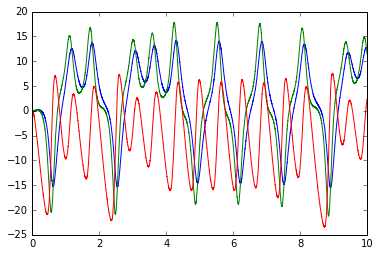
plt.figure()
plt.plot(sim.trange(), sim.data[state_probe])

[<matplotlib.lines.Line2D at 0x7fdca861fdd0>,
 <matplotlib.lines.Line2D at 0x7fdca861ffd0>,
 <matplotlib.lines.Line2D at 0x7fdca862e150>]