Nengo Example: Controlled Oscillator

The controlled oscillator is an oscillator with an extra input that controls the frequency of the oscillation.

To implement a basic oscillator, we would use a neural ensemble of two dimensions that has the following dynamics:

$$ \dot{x} = \begin{bmatrix} 0 && - \omega \\\ \omega && 0 \end{bmatrix} x $$

where the frequency of oscillation is $\omega \over {2 \pi}$ Hz.

We need the neurons to represent three variables, $x_0$, $x_1$, and $\omega$. According the the dynamics principle of the NEF, in order to implement some particular dynamics, we need to convert this dynamics equation into a feedback function:

$$ \begin{align*} \dot{x} &= f(x) \\\ &\implies f_{feedback}(x) = x + \tau f(x) \end{align*} $$

where $\tau$ is the post-synaptic time constant of the feedback connection.

In this case, the feedback function to be computed is

$$ \begin{align*} f_{feedback}(x) &= x + \tau \begin{bmatrix} 0 && - \omega \\\ \omega && 0 \end{bmatrix} x \\\ &= \begin{bmatrix} x_0 - \tau \cdot \omega \cdot x_1 \\\ x_1 + \tau \cdot \omega \cdot x_0\end{bmatrix} \end{align*} $$

Since the neural ensemble represents all three variables but the dynamics only affects the first two ($x_0$, $x_1$), we need the feedback function to not affect that last variable. We do this by adding a zero to the feedback function.

$$ f_{feedback}(x) = \begin{bmatrix} x_0 - \tau \cdot \omega \cdot x_1 \\\ x_1 + \tau \cdot \omega \cdot x_0 \\\ 0 \end{bmatrix} $$

We also generally want to keep the ranges of variables represented within an ensemble to be approximately the same. In this case, if $x_0$ and $x_1$ are between -1 and 1, $\omega$ will also be between -1 and 1, giving a frequency range of $-1 \over {2 \pi}$ to $1 \over {2 \pi}$. To increase this range, we introduce a scaling factor to $\omega$ called $\omega_{max}$.

$$ f_{feedback}(x) = \begin{bmatrix} x_0 - \tau \cdot \omega \cdot \omega_{max} \cdot x_1 \\\ x_1 + \tau \cdot \omega \cdot \omega_{max} \cdot x_0 \\\ 0 \end{bmatrix} $$

import matplotlib.pyplot as plt
%matplotlib inline

import nengo
%load_ext nengo.ipynb

<IPython.core.display.Javascript at 0x7fda1c356050>

Step 1: Create the network

tau = 0.1   # Post-synaptic time constant for feedback
w_max = 10  # Maximum frequency is w_max/(2*pi)

model = nengo.Network(label='Controlled Oscillator')
with model:
    # The ensemble for the oscillator
    oscillator = nengo.Ensemble(500, dimensions=3, radius=1.7)
    
    # The feedback connection
    def feedback(x):
        x0, x1, w = x  # These are the three variables stored in the ensemble
        return x0 + w*w_max*tau*x1, x1 - w*w_max*tau*x0, 0
    nengo.Connection(oscillator, oscillator, function=feedback, synapse=tau)
    
    # The ensemble for controlling the speed of oscillation
    frequency = nengo.Ensemble(100, dimensions=1)
    
    nengo.Connection(frequency, oscillator[2])

Step 2: Create the input

from nengo.utils.functions import piecewise
with model:
    # We need a quick input at the beginning to start the oscillator
    initial = nengo.Node(piecewise({0: [1, 0, 0], 0.15: [0, 0, 0]}))
    nengo.Connection(initial, oscillator)
    
    # Vary the speed over time
    input_frequency = nengo.Node(piecewise({0: 1, 1: 0.5, 2: 0, 3: -0.5, 4: -1}))
    
    nengo.Connection(input_frequency, frequency)

Step 3: Add Probes

with model:
    # Indicate which values to record
    oscillator_probe = nengo.Probe(oscillator, synapse=0.03)

Step 4: Run the Model

with nengo.Simulator(model) as sim:
    sim.run(5)

Step 5: Plot the Results

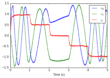
plt.plot(sim.trange(), sim.data[oscillator_probe])
plt.xlabel('Time (s)')
plt.legend(['$x_0$', '$x_1$', '$\omega$']);