Nengo Example: Unsupervised learning

When we do error-modulated learning with the nengo.PES rule, we have a pretty clear idea of what we want to happen. Years of neuroscientific experiments have yielded learning rules explaining how synaptic strengths change given certain stimulation protocols. But what do these learning rules actually do to the information transmitted across an ensemble-to-ensemble connection?

We can investigate this in Nengo. Currently, we've implemented the nengo.BCM and nengo.Oja rules.

import numpy as np
import matplotlib.pyplot as plt
%matplotlib inline

import nengo
%load_ext nengo.ipynb

<IPython.core.display.Javascript at 0x7fc78010f650>

print(nengo.BCM.__doc__)

Bienenstock-Cooper-Munroe learning rule.

    Modifies connection weights as a function of the presynaptic activity
    and the difference between the postsynaptic activity and the average
    postsynaptic activity.

    Parameters
    ----------
    theta_tau : float, optional (Default: 1.0)
        A scalar indicating the time constant for theta integration.
    pre_tau : float, optional (Default: 0.005)
        Filter constant on activities of neurons in pre population.
    post_tau : float, optional (Default: None)
        Filter constant on activities of neurons in post population.
        If None, post_tau will be the same as pre_tau.
    learning_rate : float, optional (Default: 1e-9)
        A scalar indicating the rate at which weights will be adjusted.

    Attributes
    ----------
    learning_rate : float
        A scalar indicating the rate at which weights will be adjusted.
    post_tau : float
        Filter constant on activities of neurons in post population.
    pre_tau : float
        Filter constant on activities of neurons in pre population.
    theta_tau : float
        A scalar indicating the time constant for theta integration.
    

print(nengo.Oja.__doc__)

Oja learning rule.

    Modifies connection weights according to the Hebbian Oja rule, which
    augments typicaly Hebbian coactivity with a "forgetting" term that is
    proportional to the weight of the connection and the square of the
    postsynaptic activity.

    Parameters
    ----------
    pre_tau : float, optional (Default: 0.005)
        Filter constant on activities of neurons in pre population.
    post_tau : float, optional (Default: None)
        Filter constant on activities of neurons in post population.
        If None, post_tau will be the same as pre_tau.
    beta : float, optional (Default: 1.0)
        A scalar weight on the forgetting term.
    learning_rate : float, optional (Default: 1e-6)
        A scalar indicating the rate at which weights will be adjusted.

    Attributes
    ----------
    beta : float
        A scalar weight on the forgetting term.
    learning_rate : float
        A scalar indicating the rate at which weights will be adjusted.
    post_tau : float
        Filter constant on activities of neurons in post population.
    pre_tau : float
        Filter constant on activities of neurons in pre population.
    

Step 1: Create a simple communication channel

The only difference between this network and most models you've seen so far is that we're going to set the decoder solver in the communication channel to generate a full connection weight matrix which we can then learn using typical delta learning rules.

model = nengo.Network()
with model:
    sin = nengo.Node(lambda t: np.sin(t*4))
    
    pre = nengo.Ensemble(100, dimensions=1)
    post = nengo.Ensemble(100, dimensions=1)

    nengo.Connection(sin, pre)
    conn = nengo.Connection(pre, post, solver=nengo.solvers.LstsqL2(weights=True))

    pre_p = nengo.Probe(pre, synapse=0.01)
    post_p = nengo.Probe(post, synapse=0.01)

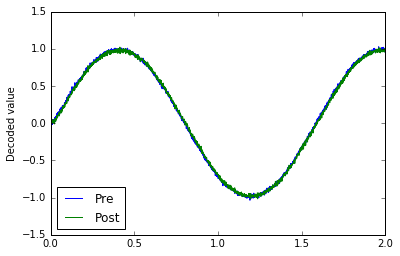
# Verify that it does a communication channel
with nengo.Simulator(model) as sim:
    sim.run(2.0)

plt.plot(sim.trange(), sim.data[pre_p], label="Pre")
plt.plot(sim.trange(), sim.data[post_p], label="Post")
plt.ylabel("Decoded value")
plt.legend(loc="best");

What does BCM do?

conn.learning_rule_type = nengo.BCM(learning_rate=5e-10)
with model:
    weights_p = nengo.Probe(conn, 'weights', synapse=0.01, sample_every=0.01)

with nengo.Simulator(model) as sim:
    sim.run(20.0)

plt.figure(figsize=(12, 8))
plt.subplot(2, 1, 1)
plt.plot(sim.trange(), sim.data[pre_p], label="Pre")
plt.plot(sim.trange(), sim.data[post_p], label="Post")
plt.ylabel("Decoded value")
plt.ylim(-1.6, 1.6)
plt.legend(loc="lower left")
plt.subplot(2, 1, 2)
# Find weight row with max variance
neuron = np.argmax(np.mean(np.var(sim.data[weights_p], axis=0), axis=1))
plt.plot(sim.trange(dt=0.01), sim.data[weights_p][..., neuron])
plt.ylabel("Connection weight");

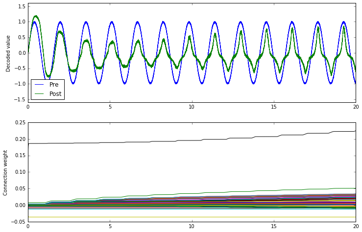
The BCM rule appears to cause the ensemble to either be on or off. This seems consistent with the idea that it potentiates active synapses, and depresses non-active synapses.

As well, we can show that BCM sparsifies the weights. The sparsity measure below uses the Gini measure of sparsity, for reasons explained in this paper.

def sparsity_measure(vector):  # Gini index
    # Max sparsity = 1 (single 1 in the vector)
    v = np.sort(np.abs(vector))
    n = v.shape[0]
    k = np.arange(n) + 1
    l1norm = np.sum(v)
    summation = np.sum((v / l1norm) * ((n - k + 0.5) / n))
    return 1 - 2 * summation

print("Starting sparsity: {0}".format(sparsity_measure(sim.data[weights_p][0])))
print("Ending sparsity: {0}".format(sparsity_measure(sim.data[weights_p][-1])))

Starting sparsity: 0.219319293771
Ending sparsity: 0.448015249982

What does Oja do?

conn.learning_rule_type = nengo.Oja(learning_rate=6e-8)

with nengo.Simulator(model) as sim:
    sim.run(20.0)

plt.figure(figsize=(12, 8))
plt.subplot(2, 1, 1)
plt.plot(sim.trange(), sim.data[pre_p], label="Pre")
plt.plot(sim.trange(), sim.data[post_p], label="Post")
plt.ylabel("Decoded value")
plt.ylim(-1.6, 1.6)
plt.legend(loc="lower left")
plt.subplot(2, 1, 2)
# Find weight row with max variance
neuron = np.argmax(np.mean(np.var(sim.data[weights_p], axis=0), axis=1))
plt.plot(sim.trange(dt=0.01), sim.data[weights_p][..., neuron])
plt.ylabel("Connection weight")
print("Starting sparsity: {0}".format(sparsity_measure(sim.data[weights_p][0])))
print("Ending sparsity: {0}".format(sparsity_measure(sim.data[weights_p][-1])))

Starting sparsity: 0.195097230164
Ending sparsity: 0.296050785009

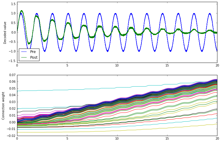
The Oja rule seems to attenuate the signal across the connection.

What do BCM and Oja together do?

We can apply both learning rules to the same connection by passing a list to learning_rule_type.

conn.learning_rule_type = [nengo.BCM(learning_rate=5e-10), nengo.Oja(learning_rate=2e-9)]

with nengo.Simulator(model) as sim:
    sim.run(20.0)

plt.figure(figsize=(12, 8))
plt.subplot(2, 1, 1)
plt.plot(sim.trange(), sim.data[pre_p], label="Pre")
plt.plot(sim.trange(), sim.data[post_p], label="Post")
plt.ylabel("Decoded value")
plt.ylim(-1.6, 1.6)
plt.legend(loc="lower left")
plt.subplot(2, 1, 2)
# Find weight row with max variance
neuron = np.argmax(np.mean(np.var(sim.data[weights_p], axis=0), axis=1))
plt.plot(sim.trange(dt=0.01), sim.data[weights_p][..., neuron])
plt.ylabel("Connection weight")
print("Starting sparsity: {0}".format(sparsity_measure(sim.data[weights_p][0])))
print("Ending sparsity: {0}".format(sparsity_measure(sim.data[weights_p][-1])))

Starting sparsity: 0.138631177963
Ending sparsity: 0.373473019429

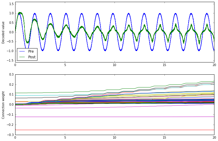
The combination of the two appears to accentuate the on-off nature of the BCM rule. As the Oja rule enforces a soft upper or lower bound for the connection weight, the combination of both rules may be more stable than BCM alone.

That's mostly conjecture, however; a thorough investigation of the BCM and Oja rules and how they interact has not yet been done.