Nengo Example: Learning a communication channel

Normally, if you have a function you would like to compute across a connection, you would specify it with function=my_func in the Connection constructor. However, it is also possible to use error-driven learning to learn to compute a function online.

Step 1: Create the model without learning

We'll start by creating a connection between two populations that intially computes a very weird function.

import numpy as np
import matplotlib.pyplot as plt
%matplotlib inline

import nengo
%load_ext nengo.ipynb
from nengo.processes import WhiteSignal

<IPython.core.display.Javascript at 0x7f530489e6d0>

model = nengo.Network()
with model:
    inp = nengo.Node(WhiteSignal(60, high=5), size_out=2)
    pre = nengo.Ensemble(60, dimensions=2)
    nengo.Connection(inp, pre)
    post = nengo.Ensemble(60, dimensions=2)
    conn = nengo.Connection(pre, post, function=lambda x: np.random.random(2))
    inp_p = nengo.Probe(inp)
    pre_p = nengo.Probe(pre, synapse=0.01)
    post_p = nengo.Probe(post, synapse=0.01)

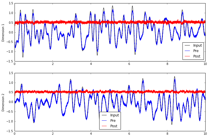
If we run this model as is, we can see that the connection from pre to post doesn't compute much of value.

with nengo.Simulator(model) as sim:
    sim.run(10.0)

plt.figure(figsize=(12, 8))
plt.subplot(2, 1, 1)
plt.plot(sim.trange(), sim.data[inp_p].T[0], c='k', label='Input')
plt.plot(sim.trange(), sim.data[pre_p].T[0], c='b', label='Pre')
plt.plot(sim.trange(), sim.data[post_p].T[0], c='r', label='Post')
plt.ylabel("Dimension 1")
plt.legend(loc='best')
plt.subplot(2, 1, 2)
plt.plot(sim.trange(), sim.data[inp_p].T[1], c='k', label='Input')
plt.plot(sim.trange(), sim.data[pre_p].T[1], c='b', label='Pre')
plt.plot(sim.trange(), sim.data[post_p].T[1], c='r', label='Post')
plt.ylabel("Dimension 2")
plt.legend(loc='best');

Step 2: Add in learning

If we can generate an error signal, then we can minimize that error signal using the nengo.PES learning rule. Since it's a communication channel, we know the value that we want, so we can compute the error with another ensemble.

with model:
    error = nengo.Ensemble(60, dimensions=2)
    error_p = nengo.Probe(error, synapse=0.03)
    
    # Error = actual - target = post - pre
    nengo.Connection(post, error)
    nengo.Connection(pre, error, transform=-1)
    
    # Add the learning rule to the connection
    conn.learning_rule_type = nengo.PES()
    
    # Connect the error into the learning rule
    nengo.Connection(error, conn.learning_rule)

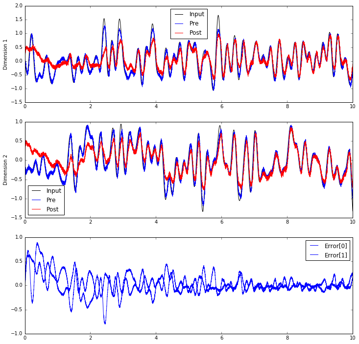
Now, we can see the post population gradually learn to compute the communication channel.

with nengo.Simulator(model) as sim:
    sim.run(10.0)

plt.figure(figsize=(12, 12))
plt.subplot(3, 1, 1)
plt.plot(sim.trange(), sim.data[inp_p].T[0], c='k', label='Input')
plt.plot(sim.trange(), sim.data[pre_p].T[0], c='b', label='Pre')
plt.plot(sim.trange(), sim.data[post_p].T[0], c='r', label='Post')
plt.ylabel("Dimension 1")
plt.legend(loc='best')
plt.subplot(3, 1, 2)
plt.plot(sim.trange(), sim.data[inp_p].T[1], c='k', label='Input')
plt.plot(sim.trange(), sim.data[pre_p].T[1], c='b', label='Pre')
plt.plot(sim.trange(), sim.data[post_p].T[1], c='r', label='Post')
plt.ylabel("Dimension 2")
plt.legend(loc='best')
plt.subplot(3, 1, 3)
plt.plot(sim.trange(), sim.data[error_p], c='b')
plt.ylim(-1, 1)
plt.legend(("Error[0]", "Error[1]"), loc='best');

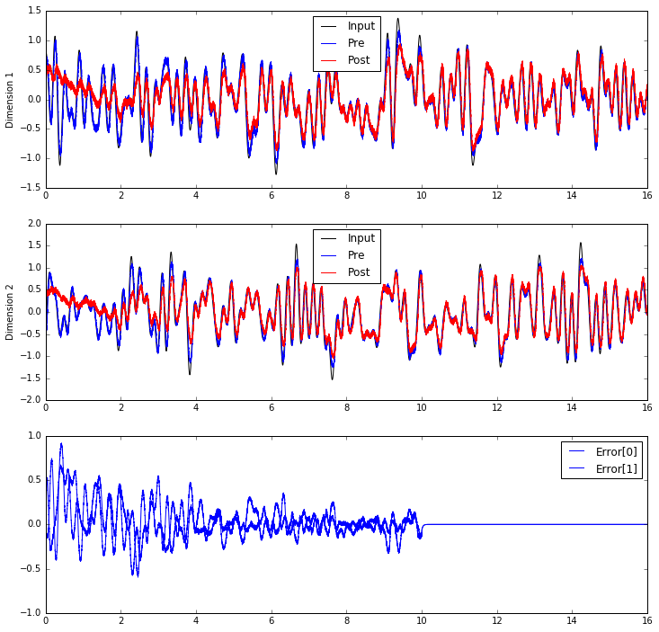
Does it generalize?

If the learning rule is always working, the error will continue to be minimized. But have we actually generalized to be able to compute the communication channel without this error signal? Let's inhibit the error population after 10 seconds.

def inhibit(t):
    return 2.0 if t > 10.0 else 0.0
with model:
    inhib = nengo.Node(inhibit)
    nengo.Connection(inhib, error.neurons, transform=[[-1]] * error.n_neurons)

with nengo.Simulator(model) as sim:
    sim.run(16.0)

plt.figure(figsize=(12, 12))
plt.subplot(3, 1, 1)
plt.plot(sim.trange(), sim.data[inp_p].T[0], c='k', label='Input')
plt.plot(sim.trange(), sim.data[pre_p].T[0], c='b', label='Pre')
plt.plot(sim.trange(), sim.data[post_p].T[0], c='r', label='Post')
plt.ylabel("Dimension 1")
plt.legend(loc='best')
plt.subplot(3, 1, 2)
plt.plot(sim.trange(), sim.data[inp_p].T[1], c='k', label='Input')
plt.plot(sim.trange(), sim.data[pre_p].T[1], c='b', label='Pre')
plt.plot(sim.trange(), sim.data[post_p].T[1], c='r', label='Post')
plt.ylabel("Dimension 2")
plt.legend(loc='best')
plt.subplot(3, 1, 3)
plt.plot(sim.trange(), sim.data[error_p], c='b')
plt.ylim(-1, 1)
plt.legend(("Error[0]", "Error[1]"), loc='best');

How does this work?

The nengo.PES learning rule minimizes the same error online as the decoder solvers minimize with offline optimization.

Let $\mathbf{E}$ be an error signal. In the communication channel case, the error signal $\mathbf{E} = \mathbf{\hat{x}} - \mathbf{x}$; in other words, it is the difference between the decoded estimate of post, $\mathbf{\hat{x}}$, and the decoded estimate of pre, $\mathbf{x}$.

The PES learning rule on decoders is

$$\Delta \mathbf{d_i} = -\frac{\kappa}{n} \mathbf{E} a_i$$

where $\mathbf{d_i}$ are the decoders being learned, $\kappa$ is a scalar learning rate, $n$ is the number of neurons in the pre population, and $a_i$ is the filtered activity of the pre population.

However, many synaptic plasticity experiments result in learning rules that explain how individual connection weights change. We can multiply both sides of the equation by the encoders of the post population, $\mathbf{e_j}$, and the gain of the post population $\alpha_j$, as we do in Principle 2 of the NEF. This results in the learning rule

$$ \Delta \omega_{ij} = \Delta \mathbf{d_i} \cdot \mathbf{e_j} \alpha_j = -\frac{\kappa}{n} \alpha_j \mathbf{e_j} \cdot \mathbf{E} a_i $$

where $\omega_{ij}$ is the connection between pre neuron $i$ and post neuron $j$.

The weight-based version of PES can be easily combined with learning rules that describe synaptic plasticity experiments. In Nengo, the Connection.learning_rule_type parameter accepts a list of learning rules. See Bekolay et al., 2013 for details on what happens when the PES learning rule is combined with an unsupervised learning rule.

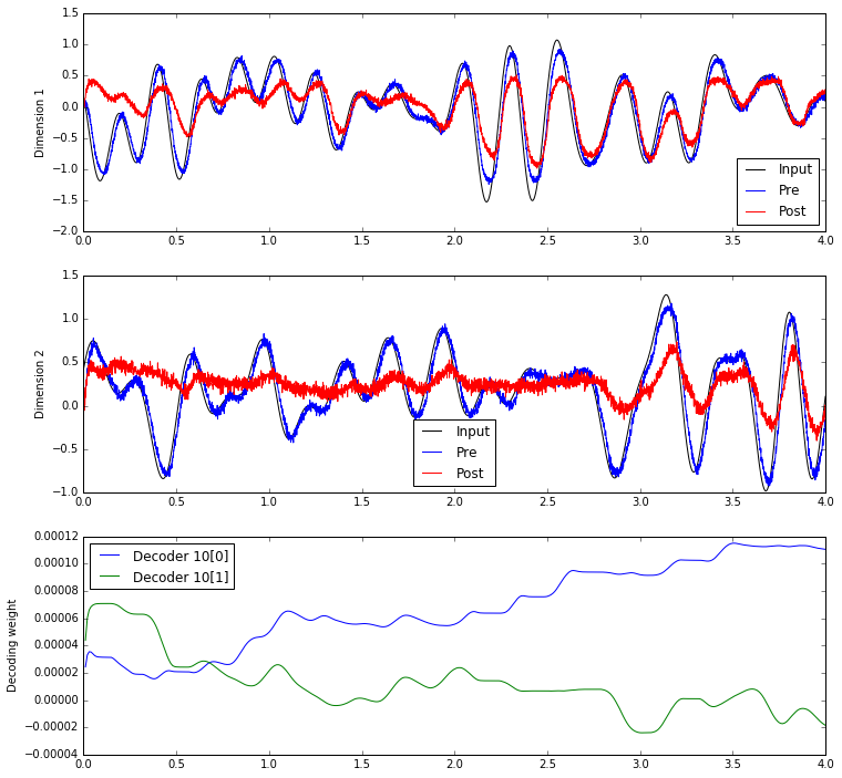
How do the decoders / weights change?

The equations above describe how the decoders and connection weights change as a result of the PES rule. But are there any general principles that we can say about how the rule modifies decoders and connection weights? Determining this requires analyzing the decoders and connection weights as they change over the course of a simulation.

with model:
    weights_p = nengo.Probe(conn, 'weights', synapse=0.01, sample_every=0.01)

with nengo.Simulator(model) as sim:
    sim.run(4.0)

plt.figure(figsize=(12, 12))
plt.subplot(3, 1, 1)
plt.plot(sim.trange(), sim.data[inp_p].T[0], c='k', label='Input')
plt.plot(sim.trange(), sim.data[pre_p].T[0], c='b', label='Pre')
plt.plot(sim.trange(), sim.data[post_p].T[0], c='r', label='Post')
plt.ylabel("Dimension 1")
plt.legend(loc='best')
plt.subplot(3, 1, 2)
plt.plot(sim.trange(), sim.data[inp_p].T[1], c='k', label='Input')
plt.plot(sim.trange(), sim.data[pre_p].T[1], c='b', label='Pre')
plt.plot(sim.trange(), sim.data[post_p].T[1], c='r', label='Post')
plt.ylabel("Dimension 2")
plt.legend(loc='best')
plt.subplot(3, 1, 3)
plt.plot(sim.trange(dt=0.01), sim.data[weights_p][..., 10])
plt.ylabel("Decoding weight")
plt.legend(("Decoder 10[0]", "Decoder 10[1]"), loc='best');

from nengo.solvers import LstsqL2
with model:
    # Change the connection to use connection weights instead of decoders
    conn.solver = LstsqL2(weights=True)

with nengo.Simulator(model) as sim:
    sim.run(4.0)

plt.figure(figsize=(12, 12))
plt.subplot(3, 1, 1)
plt.plot(sim.trange(), sim.data[inp_p].T[0], c='k', label='Input')
plt.plot(sim.trange(), sim.data[pre_p].T[0], c='b', label='Pre')
plt.plot(sim.trange(), sim.data[post_p].T[0], c='r', label='Post')
plt.ylabel("Dimension 1")
plt.legend(loc='best')
plt.subplot(3, 1, 2)
plt.plot(sim.trange(), sim.data[inp_p].T[1], c='k', label='Input')
plt.plot(sim.trange(), sim.data[pre_p].T[1], c='b', label='Pre')
plt.plot(sim.trange(), sim.data[post_p].T[1], c='r', label='Post')
plt.ylabel("Dimension 2")
plt.legend(loc='best')
plt.subplot(3, 1, 3)
plt.plot(sim.trange(dt=0.01), sim.data[weights_p][..., 10])
plt.ylabel("Connection weight");

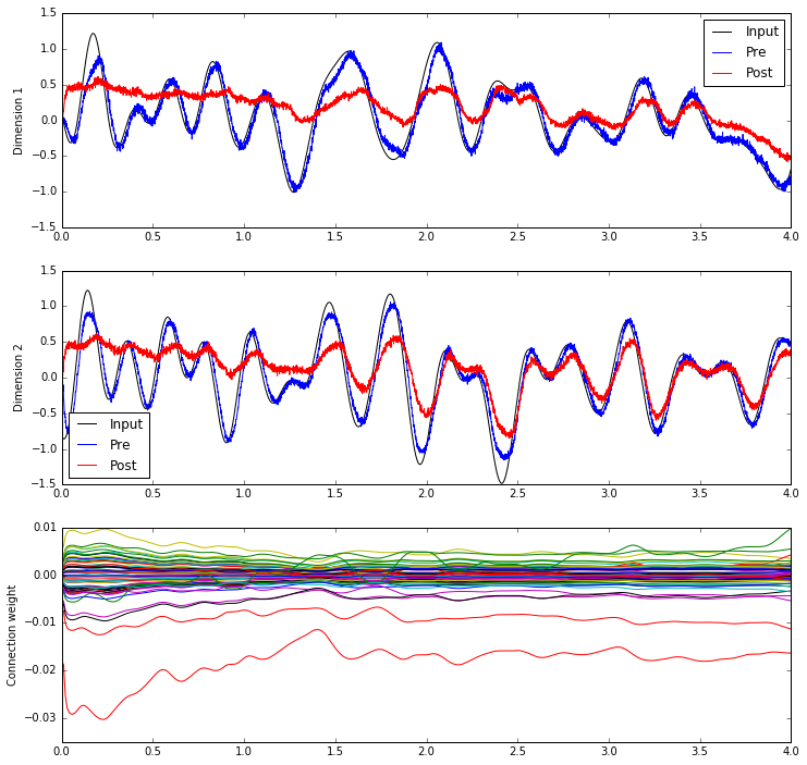
We haven't yet discovered if there are any general principles governing how the decoders and connection weights change. But, it's interesting to see the general trends; often a few strong connection weights will dominate the others, while decoding weights tend to change or not change together.